
Building a Simple Momentum Portfolio in Python: From Market Data to Backtesting
GitHub Repository
The full implementation for this project is available here: https://github.com/evangelos-com/momentum-portfolio-research
Introduction
This post walks through how a simple systematic investment idea can be implemented as a modular Python data pipeline.
The strategy here is a simple cross-sectional momentum approach (see Jegadeesh and Titman (1993)). The emphasis is on system design and implementation rather than the signal itself.
Specifically, the goal is to show how a clean engineering design can support:
- time-series data processing
- cross-sectional ranking
- portfolio construction logic
- backtesting workflows
System Overview
The system is structured into three main components:
- Signal generation
- Portfolio construction
- Backtesting engine
Each component is intentionally decoupled to improve testability and maintainability.
Data Model
The system operates on a panel dataset (a table where each row represents a specific asset at a specific point in time) with the following structure:
- date
- ticker
- price
- return
This allows both:
- time-series operations (analysis of each ticker over time)
- cross-sectional operations (comparison of all tickers at a given date)
Momentum Signal
The momentum signal is computed as a rolling percentage change over a user-defined window:
df["momentum"] = df.groupby("ticker")["price"].pct_change(window)
This produces a time-series feature representing recent price trends per asset.
A key design choice is that missing values are not removed at this stage. Instead, they are preserved for downstream handling.
Cross-Sectional Ranking
At each date, assets are ranked by their momentum score:
df["rank"] = (
    df.groupby("date")["momentum"]
    .rank(ascending=False, method="first", na_option="bottom")
)

df["selected"] = df["rank"] <= top_n
A snapshot of the ranking output for a 2020-05-27:
| Ticker | Price | Momentum | Rank | Selected |
|---|---|---|---|---|
| TSLA | 54.68 | 0.597 | 1 | True |
| NVDA | 8.49 | 0.371 | 2 | True |
| AMZN | 120.52 | 0.284 | 3 | True |
| MSFT | 173.18 | 0.100 | 4 | False |
| HD | 213.95 | 0.088 | 5 | False |
| META | 227.36 | 0.033 | 6 | False |
| UNH | 274.52 | 0.014 | 7 | False |
| AAPL | 77.07 | 0.014 | 8 | False |
| GOOG | 70.31 | -0.023 | 9 | False |
| JPM | 86.53 | -0.254 | 10 | False |
Important implementation details:
- NaN momentum values are ranked last rather than dropped
- selection is expressed as a boolean flag rather than filtering rows
NaN values occur where there is insufficient lookback history and are treated as a "pre-signal state", not missing data. They are retained, ranked last, and excluded from selection, allowing the dataset to remain structurally consistent.
As a result, the portfolio only becomes active once valid signals are available, which explains the flat section at the start of the equity curve.
Portfolio Construction
The portfolio logic is implemented as a discrete rebalancing system.
At each rebalance date:
- selected assets receive equal weights
- weights remain constant until the next rebalance date
Step 1: Initial allocation
Take the selected stocks at this rebalance date and split the portfolio equally across them.
weight = 1.0 / len(selected)
df.loc[mask, "weight"] = weight
Step 2: Weight persistence
Weights are carried forward until the next rebalance date.
The portfolio is only updated at discrete points in time and remains unchanged in between. In practice, this is equivalent to setting weights on rebalance dates and forward-filling them across subsequent days.
From an engineering perspective, this can be viewed as:
- event-driven state updates (rebalance dates)
- followed by state propagation over time
Backtesting Engine
Portfolio returns are computed by aggregating weighted asset returns.
df["weighted_return"] = df["weight"] * df["return"]

portfolio_returns = df.groupby("date")["weighted_return"].sum()
This produces a daily time series of portfolio performance.
Performance Aggregation and Benchmark Comparison
Returns are compounded to produce a cumulative performance curve:
portfolio_cum = (1 + portfolio_returns).cumprod()
The same transformation is applied to SPY (which tracks the overall market) to compare the strategy against simply buying and holding.
This ensures both the strategy and benchmark are evaluated using the same return calculation.
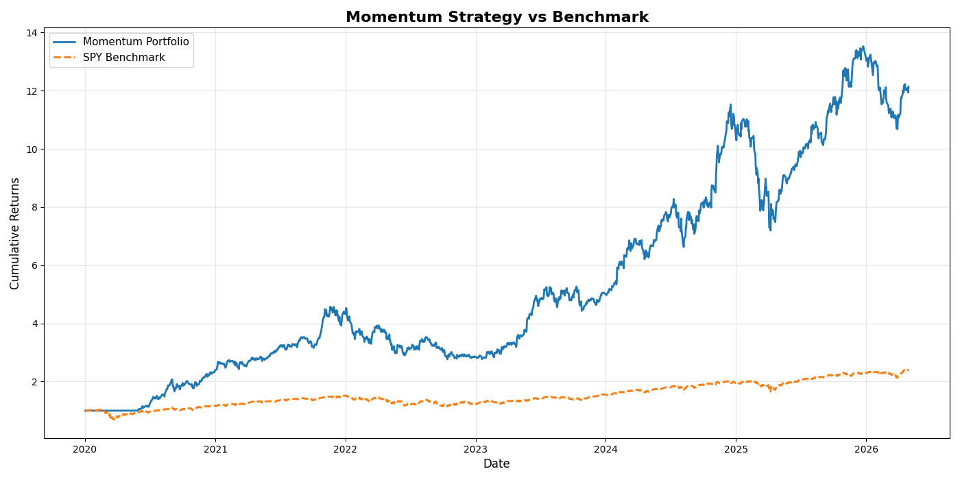
Results
Below is the resulting equity curve from the backtest:
GitHub repository: https://github.com/evangelos-com/momentum-portfolio-research
Observations
- The system implements a full data pipeline from raw prices to portfolio simulation
- The modular design allows each stage to be independently tested and modified
- Performance depends heavily on:
- the chosen asset set
- signal window
- rebalance frequency
Engineering Notes and Key Takeaways
The system is structured around three decoupled components with clear responsibilities. The SignalEngine handles signal generation and ranking, the PortfolioBuilder handles allocation logic, and the BacktestEngine focuses on performance computation. This makes each part easy to understand and modify independently.
Each step transforms a DataFrame into another DataFrame without maintaining internal state. This improves reproducibility and makes debugging more straightforward.
Portfolio weights are carried forward between rebalance dates so that each day has an explicit view of the portfolio composition. This makes it easy to inspect how the portfolio evolves over time.
More broadly, this project highlights that financial workflows are essentially data engineering problems, which is fun for me! At their core, they involve transformations over time-series datasets, grouping operations across entities, and state propagation through time.
Running the full backtest shows that the pipeline is lightweight in practice. The process uses around 350 MB of RAM, indicating that Pandas is sufficient for this research-scale workload under the current design.
Conclusion
This project demonstrates how a simple momentum-based strategy can be implemented as a clean, modular Python system.
While the strategy itself is intentionally basic, the architecture reflects patterns commonly used in production financial data systems:
- ETL-style preprocessing
- signal generation and ranking pipelines
- stateful portfolio construction
- time-series aggregation
The full code is available here: https://github.com/evangelos-com/momentum-portfolio-research
Extra Note
This mini blog is built with Next.js, TypeScript, and React.